|
|
|
 |
|
|
The means by which nerves conduct impulses have been puzzling researchers for centuries. The electrical nature of the impulse was first suspected by Luigi Galvani in 1780, when he caused the leg of a frog to contract after stimulating it with an electric charge from the newly developed Leyden jar. In the nineteenth century, Emil Du Bois Reymond first demonstrated the action potential and later wrote, "If I do not greatly deceive myself, I have succeeded in realizing (albeit under a slightly different aspect) the hundred years dream of physicists and physiologists, to wit, the identity of the nervous principle with electricity." Later, in 1902, Julius Bernstein postulated the "membrane theory" of the nerve impulse, when he proposed that the impulse is related to changes in the ion permeability of the membrane. Finally much of our present knowledge concerning the events associated with the action potential and the nerve impulse is based on the ingenious work with the giant axon of the squid performed by Hodgkin and Huxley in England and Curtis and Cole in the United States during the late 1940s and early 1950s.
Neurons are ideally suited to function as the information-carrying units of the nervous system. The length of their individual processes varies from a fraction of a millimeter in the brain to axons over 1 m in length in the spinal cord and peripheral nerves. The information-carrying signal that travels along the neuron is an electrical event called the impulse. All impulses which a neuron conducts are nearly alike. Therefore the information which a neuron can transmit is determined by the firing pattern as well as the number of impulses per second (IPS) it sends. Neurons can vary their impulse firing rates from 0 to just over 1000 IPS. Because neurons have such a wide range of firing rates and patterns they can transmit considerably more information to the brain than they could if all they had was a simple "on-off" system. For those functions in which speed of action is biologically important, neurons with high conduction velocities are often employed. Neurons with considerably slower conduction velocities are often found in neural circuits which do not require such speed. Conduction velocity is an inherent property of the neuron, increasing with fiber diameter and the degree of myelination. In mammalian neurons, conduction velocities vary anywhere from 0.2 up to 120 m/s. Nervous systems are incredibly complex networks of nerve cells in which impulses traveling along one neuron initiate impulses in other neurons at chemically responsive junctures called synapses. Chemicals called neurotransmitters are released at these synapses in response to the "arrival of impulses at the presynaptic terminals of the first neuron. When impulses arrive at a sufficient number of these presynaptic terminals, enough neurotransmitter is released to stimulate the postsynaptic neuron to its excitation threshold. When this happens there occurs on the membrane of the postsynaptic neuron a rapid and reversible change called an action potential. Once initiated this action potential generates a small local current which initiates a second action potential on the adjacent membrane segment. The local current from this action potential will, in turn, initiate a third, and so on down the entire length of the axon to the very ends of its terminal branches. Although the action potential is actually reinitiated by this series of events, we generally speak as though its propagation is a continuous smooth process. This series of propagated action potentials constitutes the impulse, and represents the signal which forms the basis for the information which the nervous system conducts.
When neurons conduct impulses, electrical currents flow through their membranes and it is therefore not possible to understand the former without a working knowledge of the latter. Besides, electronic instruments are used to record action potentials and impulses, and neurophysiologists commonly employ electrical terms and symbols in describing neuronal events. So it is actually well worth to review a few basic principles of electricity which are critical to the understanding of nerve cells.
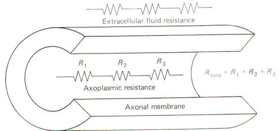
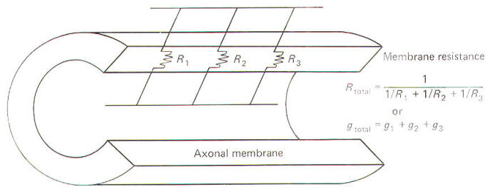
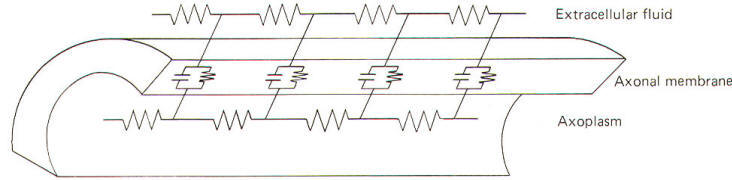
All conducting media offer some degree of resistance to the passage of current whether carried by electrons or by ions. The unit of resistance R is the ohm (Ω). It represents the resistance of a conductor such that a constant current of one ampere requires a potential of one volt between its ends. All things being equal, current follows the path of least resistance in any circuit. Neurophysiologists also use a related value called conductance g. It represents the reciprocal of resistance. The unit of conductance is the siemen (S). However, the earlier term mho (ohm spelled backward) is commonly used in most of the classical literature. Because of this reciprocal relationship, all statements concerning resistance are reciprocally related to conductance. g=1/R where g = conductance, S and R = resistance, Ω Concerning resistance are reciprocally related to conductance. Neurophysiologists are often concerned with the total resistance in several resistive elements. Neuronal membranes behave in part as if they were composed of parallel resistive elements, while the extracellular and intracellular fluids surrounding the membrane behave like series resistors. Since electric currents flow through the membrane and both of these fluids during impulse conduction, it is important to be able to estimate the total resistance involved. Biologically, the important point to remember here is that the total resistance of series resistors is equal to their sum, but the total resistance of parallel resistors is equal to a value less than their sum. Fig-2 illustrates the series resistive nature of the axoplasm and extracellular fluid, while Fig-3 pictures the axonal membrane in the form of parallel resistors.
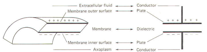
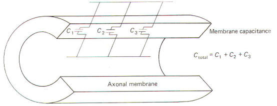
The neuronal membrane behaves in part as if it were composed of parallel capacitors. A capacitor is a charge-storing component consisting of two conductors separated by a dielectric (insulator). The membrane represents the dielectric while the extracellular fluid and the axoplasm represent the conductors (Fig-4). The unit of capacitance C is the farad (F). It represents the capacitance of a capacitor in which a charge of one coloumb produces a potential difference of one volt between the terminals (conductors). The relationship between capacitance (in farads) and the potential difference (in volts) produced by a given charge separation (in coulombs) is given by C= Q/V where C = capacitance, F Q = charge, C V = potential, V By manipulation of the equation we can see that the charge that needs to be separated in order to produce a specific voltage is given by: Q=CV Similarly, the potential developed by the transfer of a given charge across a capacitance is given by: V= Q/C Neurophysiologists are generally concerned with the total capacitance in a section of membrane. Since the neuronal capacitance is only associated with the membrane, we need not concern ourselves with other aspects of the neuron, Because the membrane behaves as if it were in part composed of parallel capacitors, we are interested in the rules governing parallel capacitors (Fig-5).
The unit of potential E is the volt (V). The difference in potential between two points is related to the work done in moving a point charge from the first point to the second. It is equal to the difference in the value of the potentials at the respective points. Biologically important voltages are usually quite small, in the order of millivolts (mV) or microvolts (µV). In simple direct current (dc) wire circuits, the battery is an electronic component which represents a potential difference as well as a source of charge (electrons). In neurons, ions represent the charge while the chemical (concentration) gradient for a given ionic type represents the potential for that ion. The relationship between potential, current, and resistance is expressed by Ohm's law: I=E/R where I = current, A E = potential, V R = resistance, Ω In neuron studies we are often concerned with conductance. Consequently a useful form of the equation is: I =Eg where g = conductance, S
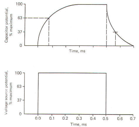
Functionally a capacitor can do three things. It can become charged, it can store a charge, and it can discharge. When a capacitor is connected to a voltage source, current will flow and build up charges on one side of the capacitor while removing them from the other side in the process of completing the circuit. Current will flow in the circuit only until the charge on the capacitor attains the same potential as the voltage source. At the point the capacitor is fully charged, current will no longer flow in the circuit. A resistor is usually pictured as being in series with the capacitor in such a circuit - hence, the name resistance-capacitance (RC) circuit. If the voltage source is removed and the charged capacitor and resistor are connected in a closed loop, current will once again flow as charges are drawn off the capacitor through the resistor to equalize on both sides of the dielectric. Thus the capacitor is discharged and the potential removed. This current which flows only when the capacitor is being charged or discharged is called capacitive current Ic . It is proportional to the rate of change of voltage across the capacitor. All physical systems require a certain amount of time to transmit given quantities of charge from input to output. This time in simple RC systems is characterized by the system time constant t. It is mathematically equal to the product of the resistance (in ohms) and the capacitance (in farads). The resultant time constant is in seconds and represents the time required for the voltage to reach 1 -1/e (63 percent) of its final value. The symbol e is the base of the natural logarithm (2.71828"'). t=RC where t = time constant, s R = resistance, Ω C = capacitance, F When a voltage source is suddenly applied across an uncharged RC circuit, there is a delay in the rise of the potential developed on the capacitor, which is accounted for by the time required to store charges (Fig-6). The time constant represents the time in seconds it takes for the capacitor to produce a voltage 63 percent as high as its final value when it is fully charged. Similarly, when the capacitor is discharged, it takes just as long (i.e., one time constant) for the capacitor to lose 63 percent of its charge.
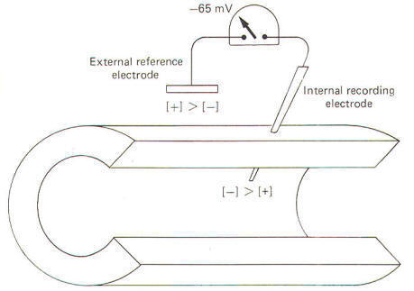
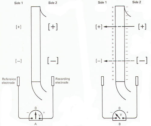
All cells exhibit an electrical potential across their membranes called a membrane potential (MP). However, nerve and muscle cells are somewhat unique in that this membrane potential can be reduced (depolarized) or increased (hyperpolarized) as a result of synaptic activity. This feature makes nerve and muscle cells excitable. When a neuron is not being stimulated its membrane potential is relatively stable and is therefore referred to as a resting membrane potential (RMP). A typical RMP for mammalian nerve and muscle cells lies between 70 and 100 mV, with the intracellular fluid negative. For illustrative purposes consider a common average for a large mammalian nerve cell axon of -85 mV with the dendritic zone (soma and dendrites) being less polarized at approximately -70 mV. Much of what we believe today concerning membrane potentials and action potentials is based on experiments with the giant axon of the squid. Such studies laid the groundwork for almost all of our present assumptions concerning nerve excitability. Accordingly, many of the examples included here will be based on action potentials and impulses in the squid axon. When a squid or mammalian nerve axon is penetrated by a recording micro electrode and the internal potential compared to an external reference electrode, the axoplasm is found to be negative with respect to the outside. The magnitude of this potential is about -65 mV in the squid. The obvious assumption which can be made is that there are slightly more positive than negative charges outside, and slightly more negative than positive charges inside (Fig-7).
How important is it for nerve cells to have a resting membrane potential? Quite simply, without it (1) they would not be excitable, (2) they could not produce action potentials, and (3) they could not conduct impulses. Thus because of its important role in the impulse conducting process, a good place to start our discussion is with the origin of the RMP itself.
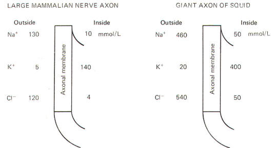
Julius Bernstein demonstrated in the early 1900s that ionic fluxes across the membrane were important to the impulse-conducting capabilities of neurons. He demonstrated that resting membranes were typically more permeable to K+ ions than they were to Na+ ions. Typical extracellular and intracellular concentrations of Na+, K+, and Cl- in a large mammalian nerve cell axon and the giant axon of the squid are illustrated in Fig-8.
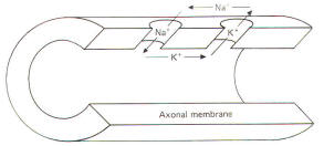
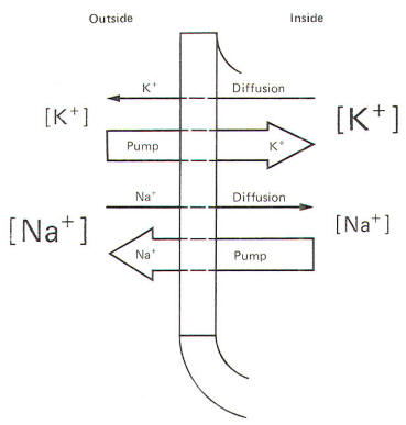
Even a quick observation of the various concentrations in Fig-8 shows us that Na+ and Cl- are much more concentrated extracellularly, while K+ is much more concentrated intracellularly. The membrane which separates these two solutions in both the squid and mammalian cells is freely permeable to water but is much less permeable to the above-listed ions. Not depicted in Fig-8 are the nonpermeable anions found within the intracellular fluid. These anions are composed primarily of large protein molecules. Because of the free permeability of the membrane to water, the inside and outside solutions have virtually the same osmolality. Even though the membrane is not very permeable to either cation listed in Fig-8, recall that Bernstein showed the resting membrane to be more permeable to K+ than to Na+. It was subsequently discovered that CI- permeates more readily than K+ in the mammalian axon and less readily than K+ in the giant axon of the squid. The membranes of both species actively transport Na+ to the outside and K+ to the inside. Hence the tendency for the ions to diffuse down their chemical gradients is counterbalanced by the Na+ and K+ active transport system (Na+/K+ "pump") transporting these ions against their chemical gradients (Fig-9).
When a cell is at rest it obeys two basic principles, the principle of equimolality and the principle of electrical neutrality. These two principles are summarized here. 1 The
principle of equimolality. The concentrations of osmotically
active particles on both sides of the cell membrane should be
approximately equal. Chemical analysis of the solutions on each side of the two types of nerve cells verifies that these two principles are essentially true. A second examination of the ionic distributions will show that the high extracellular concentration of Na+ is primarily balanced by the high extracellular concentration of Cl-, while the high intracellular K+ concentration is primarily balanced by the high intracellular concentration of large nonpermeating anions we referred to earlier. We have neglected to list other such ions as Mg2+ , Ca2+, and several others which are also present in the solutions on either side. Their concentrations are small and otherwise unimportant in the events of the action potential and impulse. Nevertheless they help to contribute to the principles of equimolality and electrical neutrality. You might well be wondering how it is possible to have a resting membrane potential if the solutions on both sides of the membrane are electrically neutral. The answer lies in the fact that the principle of electrical neutrality is only approximately true. As we have previously noted (Fig-7) there are actually slightly more cationic than anionic charges outside and slightly more anionic than cationic charges inside. This slight imbalance, or violation of the principle of electrical neutrality, is sufficient to produce the potential difference across the resting membrane. As we will see later an imbalance of only a few picomoles (10-12 mol) is sufficient to produce the resting membrane potential
A relatively simple experiment might be helpful in understanding how the resting membrane potential develops. If you were to place a highly concentrated salt solution on one side of a selectively permeable membrane and a less concentrated solution on the other side, the salt would diffuse through the membrane from the highly concentrated to the less concentrated side until it reached equilibrium. Now if the membrane was more permeable to the cation of the salt than it was to the anion, positive charges would migrate to one side faster than negative charges and a charge separation would develop across the membrane with one side more positive than the other (Fig-10). A sensitive voltmeter applied across the membrane would register a potential difference, and because this potential is caused by unequal diffusion rates it can properly be called a diffusion potential.
The resting membrane potential which exists in both the mammalian and squid axons is thought to be primarily due to a diffusion potential caused by the charge separation which results as K+ ions diffuse outward down their concentration gradient, leaving the large nonpermeating anions behind.
As K+ ions diffuse outward following their chemical (concentration) gradient, the outside of the membrane becomes increasingly positive while the inside becomes more negative. This continual tendency for K+ to diffuse outward is increasingly opposed by the buildup of an electrical gradient in the opposite direction, from outside to inside. That is, the increasing positivity on the outside opposes the further flow of positively charged K+ outward, and the increasing negativity of the inside surface of the membrane tends to restrict the escape of K+. When the electrical gradient has increased to a point where it is sufficient to stop the net outward flow of K+, the ion is said to be at electrochemical equilibrium. The relationship between the concentration gradient across the membrane of any given ion and the membrane potential which will just balance it at electrochemical equilibrium is given by the physiochemical relationship known as the Nernst equation. It represents the equilibrium potential for that particular ionic type. The Nernst equation is commonly used in one of two forms. The second equation, derived from the first, is often preferred because it is easier to work with and suffers little loss in accuracy. E= RT/zF InC1/C2 (2-1) E= 58 logC1/C2 (2-2) where E = equilibrium potential [expressed in volts in Eq. (2-1) and millivolts in Eq. (2-2)]. R = universal gas constant, 8.32 J mol-1 K-1 . z = valence and charge of ion. F = Faraday constant, 96,500 C/mol. C1/C2= chemical gradient. In= natural logarithm. log= common logarithm. 61 is used if preparation is at body temperature (37oC); 58 is used if preparation is at room temperature (20oC). The equilibrium potentials calculated by these equations are slightly different for each nerve cell depending on whether Eq. (2-1) or Eq. (2-2) is used. This is due to rounding errors in converting the quantity (RT/ zF) In to the quantity 61 log or 58 log. However, for all practical purposes, the error is quite small and can be ignored. The Nernst equation is interpreted this way. In the squid axon, K+ is 20 times more concentrated inside than outside and therefore has a chemical gradient directed outward. It would require an external positivity of about 76 mV (internal negativity equal to -76 mV) to just balance this gradient at electrochemical equilibrium and stop the net diffusion of K+ outward. Since the RMP of the squid axon isn't quite this negative inside, there is a continual tendency for K+ to diffuse outward. Now consider that a cation gradient from inside to outside and an anion gradient from outside to inside will be balanced at electrochemical equilibrium by internal negativity. Similarly, a cation gradient from outside to inside and an anion gradient from inside to outside will be balanced by internal positivity. Consequently, the following forms of the Nernst equation can theoretically predict both the magnitude and polarity of the internal potential: E = - 58 log (cationi/cationo) E = -58 log (aniono/anioni)
The equilibrium potential necessary to just balance a given chemical gradient can be theoretically predicted by the Nernst equation. The values for the mammalian nerve cell and the squid axon are listed below. Large
mammalian nerve cell ENa+ = 68 mV Giant axon
of the squid ENa+ = 56 mV Remember that the RMP of the large mammalian nerve cell is -85 mV, while it is about -65 mV in the giant axon of the squid. Since the equilibrium potentials for K+ and Na+ listed above are not the same as the resting membrane potentials, it follows that neither K+ nor Na+ is really at electrochemical equilibrium in the large mammalian nerve cell nor in the giant axon of the squid. Any time that an ion is not in electrochemical equilibrium, net diffusion of that ion will occur and the chemical gradient will change unless some other factor such as membrane active transport acts to restore the gradient. Of course, in the nerve cells described here, the Na+/K+ pump does just that, and their respective chemical gradients are maintained.
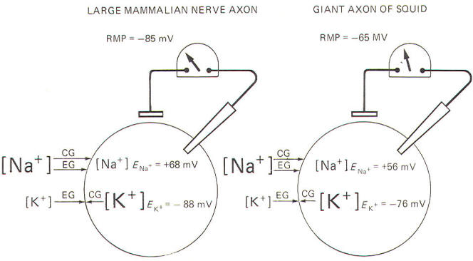
Neither Na+ nor K+ is in electrochemical equilibrium across the resting membrane of the mammalian neuron and the giant axon of the squid (Fig-11).
For Na+, notice that both the chemical and electrical gradients are directed inward. In order to be in equilibrium, the inside would need to be about +68 mV in the mammalian neuron, and about +56 mV in the squid. And we know by intracellular microelectrode recording that both interiors are actually negative in the resting membrane. In the case of K+ ions, the electrical gradient is directed inward while the chemical gradient is directed outward because of relatively high intracellular K+ concentration. The inside would need to be about -88 mV in the mammalian neuron and about -76 mV in the squid in order for K+ to be in electrochemical equilibrium. Notice that the experimentally measured RMP is very close to these values in each case. That is, EK+ = -88 mV compared to an RMP of -85 mV in the large mammalian nerve axon, and EK+= -76 mV compared to an RMP of -65 mV in the giant axon of the squid. It is apparent that K+ is almost in electrochemical equilibrium across the resting membrane of both cells. Nevertheless, the respective potassium equilibrium potentials are slightly more negative than their resting membrane potentials. Consequently, there is a continual tendency for K+ ions to diffuse outward.
You might be wondering at this point how the Na+/K+ "pump" fits into the picture. Earlier, we noted that both the electrical and chemical gradients for sodium are directed inward. In addition, while the membrane is not easily penetrated by Na+, some ions will nevertheless cross. Why then doesn't Na+ simply diffuse down its two gradients and reach equilibrium on each side of the membrane? The answer lies in the capability of the cell membrane to actively transport (pump) Na+ outward, against these two gradients. Not all of this actively transported Na+ stays outside, however, since a small amount leaks back inward because of the slight permeability of the membrane to this ion. One can readily appreciate, however, that the outward Na+ transport and the inward Na+ diffusion must match each other in effectiveness since there is no net change in the extracellular and intracellular concentrations of this ion during the time that the membrane is in the resting state. As far as K+ is concerned, remember that the chemical gradient is outward while the electrical gradient is inward. This inward electrical gradient coupled with the fact that the membrane actively transports K+ to the inside accounts for the high intracellular K+ concentration found in both cell types. Once again, not all of the actively transported K+ which is pumped inward stays inside. Because of the outward-directed chemical gradient and the limited permeability of the membrane to this ion, some K+ diffuses outward. The membrane of the resting mammalian nerve axon is typically 100 times more permeable to K+ than to Na+, while in the squid axon a 25:1 ratio is observed. Nevertheless, the inward pumping and outward diffusion of K+ must once again match each other since there is no net change in the inside and outside concentrations of this ion during the time the membrane is in the resting state.
In the resting membrane, none of the cations and anions in the solutions on either side of the membrane are at electrochemical equilibrium. Consequently, they are diffusing across the membrane with different diffusion rates and in different directions at all times in the resting membrane. The only time an ion won't diffuse is when (1) it is at electrochemical equilibrium or (2) the membrane is not permeable to it at all. Consequently a variety of charge separations are occurring simultaneously across the membrane, with each contributing to a greater or lesser extent to the experimentally measured resting membrane potential. Hodgkin and Katz, using a formula developed earlier by Goldman, attempted to theoretically predict the resting membrane potential by considering the combined effects of all these ions including (1) the ionic charge, (2) the direction of the chemical gradient, and (3) the relative permeability of the membrane to each. VM = -58 log { [Na+]i PNa+ + [K+]i PK+ + [CI-]o PCl- }/{[Na+]o PNa+ + [K+]o PK+ + [CI-]i PCl-} where VM = membrane potential, mV. Pion = membrane permeability for a given ion. The accuracy of this equation in predicting actual resting membrane potentials is dependent on the permeability factors for each ion which are only close approximations of their true values. Nevertheless, the predicted values are usually quite close to the measured RMPs. Careful examination of this equation will show several things. First notice that the Goldman-Hodgkin-Katz equation is an extension of the Nernst equation. Since it considers the collective contributions of Na+, K+, and CI- chemical gradients as well as the relative permeability of the membrane to each, the integrated equilibrium potential which the equation predicts is at least theoretically a close approximation of the RMP itself. The theoretical prediction which this equation makes for the RMP of the large mammalian nerve cell at body temperature and the giant axon of the squid at room temperature is given below. Large mammalian nerve cell VM = -61 log (0.01) +1400(1) + 120(2)/ 130(0.01)+ 5(1) + 4(2) = -87 mV Giant axon of the squid VM = - log 50(0.04) + 400(1) + 540(0.45) /460(0.04) + 20(1) + 50(0.45) =-59 mV
Earlier we noted that when a single area of axonal membrane is stimulated it becomes excited and undergoes a rapid and reversible electrical change called an action potential. And recall further that this action potential propagates as a continuous impulse down the entire length of the axon. Let's now examine the changes which occur in the neuron during the action potential. The action potential results from a sudden change in the resting membrane potential (a condition necessary for impulse conduction). To illustrate this point, it is usually convenient in experimental laboratory conditions to stimulate the neuron at some point on its axon. You should recognize that this is not a normal situation. Neurons are rarely stimulated on their axons in vivo. Instead they are stimulated to produce action potentials in vivo via (1) generator potentials from sensory receptors, (2) neurotransmitters from presynaptic terminals at synapses, and (3) local currents. Nevertheless, an action potential is still an action potential no matter where or how it is produced and the axon is generally much more accessible in experimental situations than is the rest of the neuron. By this time you should be aware that the resting membrane is a polarized membrane. That is, unlike charges are separated at the membrane with the inside negative and the outside positive. When the membrane is stimulated by an electronic stimulator in the laboratory, its resting membrane potential begins to decrease. That is, it becomes less negative and hence less polarized. If it is depolarized to a critical level known as the excitation threshold, an action potential will be produced at the point of stimulation. Once the membrane potential is depolarized to the excitation threshold, its Na+ channels (routes through which Na+ ions cross the membrane) suddenly open and a tremendous increase in Na+ conductance g",,+ occurs with Na+ ions now free to diffuse down both their chemical and electrical gradients. This is called sodium activation. You should note that conductance g is the electrical analog of permeability P. Thus it is also appropriate to say that there is a sudden and marked increase in sodium permeability on the part of the membrane when the excitation threshold is reached. As the positively charged Na+ ions suddenly diffuse inward the RMP is greatly disturbed at the local site of stimulation. Sufficient positively charged Na+ is removed from the immediate membrane exterior surface and transferred to the immediate membrane interior surface to totally eliminate the internal negativity and replace it with positivity. Measurement now would record a reversed potential showing the interior now positive with respect to the exterior. We will see later that only a few picomoles of Na+ actually need to diffuse inward to change the membrane potential by 125 mV, that is, from a RMP of -85 mV to a reversed potential of +40 mV in the large mammalian neuron or a RMP of -65 mV to a reversed potential of +55 mV in the giant axon of the squid. This local reversed potential is not allowed to last. Even before the intracellular fluid reaches its maximum positivity, the local membrane channels for K+ open, causing a great increase in membrane permeability to K+ with a resulting increase in gK+ and carrying positive charges to the outside down their chemical and electrical gradients. At the same time there is a marked reduction in gNa+. This coupled with the substantial increase in K+ outflow is sufficient not only to eliminate the internal positivity caused by the Na+ inflow, but also to actually restore the original resting membrane potential. It is important to understand that the depolarization caused by the Na+ inflow and the repolarization caused by the K+ outflow occur locally. That is, they occur only on that section of axon which is initially stimulated. The entire action potential, including depolarization to the reversed potential and repolarization back to the resting membrane potential, happens very quickly, requiring no more than a few milliseconds.
The capacitance of a typical nerve cell membrane has been estimated to be 1 µF/cm2 Therefore the number of charges which need to be transferred across the membrane capacitor to change its potential by 125 mV is given by Q=CV = (10-6 F/cm2) (1.25 x 10⁻¹ V) . = 1.25 X 10⁻⁷C/cm2 Now the number of sodium ions which need to diffuse inward in order to transfer 1. 25 x 10-7C of charge from the extracellular fluid, through one square centimeter of membrane, to inside can be calculated from the Faraday constant. Number of moles transferred per square centimeter = membrane charges transferred per square centimeter x (1/ Faraday constant ) = (1.25 X 10⁻⁷C/cm2) (1 x 10⁻⁵ mol/C) = 1.25 x 10⁻¹² mol/cm2 = 1.25 pmol/cm2 These few picomoles which diffuse inward during the depolarization of the membrane to the reversed potential stage are so insignificantly few in a largediameter nerve fiber that they cause virtually no change in the measurable extracellular or intracellular sodium concentrations. Similarly, the outward diffusion of 1.25 pmol of K+ per square centimeter is sufficient to repolarize the membrane back to the resting level, and yet this loss of intracellular K+ is so insignificant as to leave virtually unchanged the extracellular and intracellular K+ concentrations. Of course, the smaller the fiber the greater will be the change in the intracellular concentrations of these ions. But still the change would be insignificantly slight. In any event, the nerve cells are constantly being recharged by active transport outward of the few picomoles of Na+ which diffuse inside during depolarization, and by actively transporting inward the few picomoles of K+ which diffuse outward during depolarization. Recharging enables neurons to conduct virtually unlimited numbers of impulses without producing changes in the ionic concentrations which are vital for maintaining their excitability. As a theoretical exercise you can calculate the small percentage of internal K+ which needs to diffuse outward in order to repolarize the membrane by considering the axon to be a cylinder of uniform diameter. For example, consider a large mammalian nerve axon with a diameter of 20 µm (2 x 10⁻³ cm) and an intracellular concentration of K+ equal to 140 mmol/L. Percent of intracellular K+ diffusing out = (number of moles of K+ diffusing out through a given length of axon / number of moles of K+ in axoplasm for a given length of axon) x 100 = {[(moles diffusing out)/(cm2 of membrane)](cm2 of membrane) / (mol/cm2 of axoplasm)} x 100 = {(1.25 x 10⁻¹² mol/cm2) [277(1 X 10⁻¹ cm)] (cm) / (1.4 X 10⁻⁴ mol/cm2) [77(1 x 10⁻¹ cm)2](cm)} x 100 =(7.9 x 10⁻¹⁵ mol / 4.4 X 10⁻¹⁰ mol ) x 100 = 1.8 x 10⁻³ percent During the remainder of our discussion on the events associated with the action potential we will examine exclusively the work done with the giant axon of the squid. You really lose nothing by abandoning for the moment the mammalian axon in favor of concentrating on the squid axon. In fact. quite to the contrary, you get a real feel for the work of Hodgkin and Huxley in developing the principles we accept so easily today.
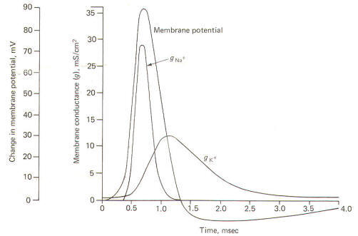
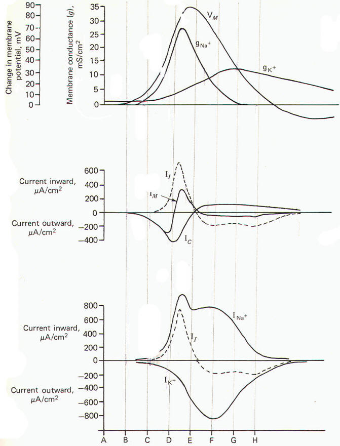
Using a technique called the voltage clamp, Hodgkin and Huxley calculated the time course of sodium and potassium conductance. g"o~ and gl(~' as well as sodium and potassium current, I"" T and I I( ~, during an action potential. We will examine this technique later, but for the moment consider the calculated relationships with time during the action potential illustrated in Fig-12.
The action potential pictured here underwent a sudden but reversible change in its membrane potential. Notice that the initial value of the RMP and the final value of the reversed potential are not indicated. Instead all we see is the magnitude of depolarization from the former to the latter. Notice that when the membrane potential has depolarized by about 10 mV (presumably to the excitation threshold) there is a sudden and large increase in gNa+ to about 30 mS/cm2 This is responsible for the large and sudden change in the membrane potential. Notice further that this large increase in g"" - is transient and the conductivity returns within a few milliseconds to practically zero. Meanwhile a slower increase in the gK+ to about 12 mS/cm2, which started even before the membrane potential reached its maximum reversed potential. promotes the repolarization of the membrane. Consequently the membrane potential changes once again back to the resting level. In fact the membrane often hyperpolarizes beyond the resting level by a few millivolts before gradually returning to the resting level after several milliseconds. This slow return to the resting level is called the afterpotential. The rapid rise and fall in membrane potential is called the spike or spike potential. However, the action potential includes both the spike potential and the afterpotential.
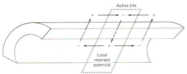
During the reversed potential the axoplasm immediately inside the stimulated area of membrane is temporarily made positive while the adjacent axoplasm is still negative. Similarly the extracellular fluid immediately outside the stimulated area is temporarily negative while the adjacent extracellular fluid is still positive. Thus charge gradients exist side by side and a small current begins to flow in a circuit through the membrane. The direction of this current is inward through the depolarized areas, laterally through the adjacent axoplasm, outward through the adjacent still-polarized membrane segment immediately adjacent to the depolarized area, laterally backward through the extracellular fluid, and inward once again through the depolarized area. The path of this local current is illustrated in Fig-13.
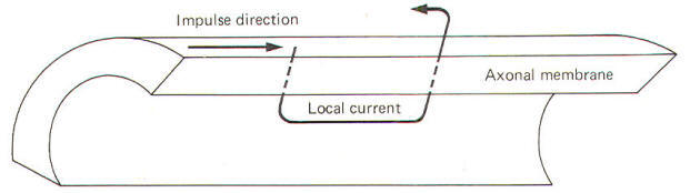
As the local current flows outward through the adjacent still-polarized membrane, the membrane at this point begins to depolarize. Once it has depolarized to the excitation threshold, the sodium channels suddenly open and the resultant increase in gNa+ causes the now-familiar action potential to occur at that point on the membrane. Subsequently, as this new action potential develops, a new local current will flow from it to the next adjacent membrane segment, depolarizing it and propagating a continuous impulse down the axon. Of course if the axon is stimulated at some point along its length the local current will spread in both directions away from the stimulus site and an impulse will travel in both directions. You should always keep in mind that this condition (impulse spread in both directions) occurs only in the laboratory preparations when neurons are stimulated along their axons. As we pointed out earlier, neurons are rarely stimulated on their axons in vivo. Instead they are stimulated in dendritic zones to produce action potentials via generator potentials from sensory receptors and neurotransmitters from presynaptic terminals at synapses. In axons, local currents traveling ahead of propagated action potentials are responsible. In all these naturally occurring stimulus situations, the local currents and hence the propagated action potentials travel in only one direction. This direction is toward the terminal branches of the axon. Approximately 0.5 ms after the local area of membrane depolarizes, it starts to repolarize as a result of the progressive increase in gK+ . Thus the impulse which travels down an axon is followed about 0.5 ms later by a wave of repolarization as each succeeding membrane segment begins to repolarize.
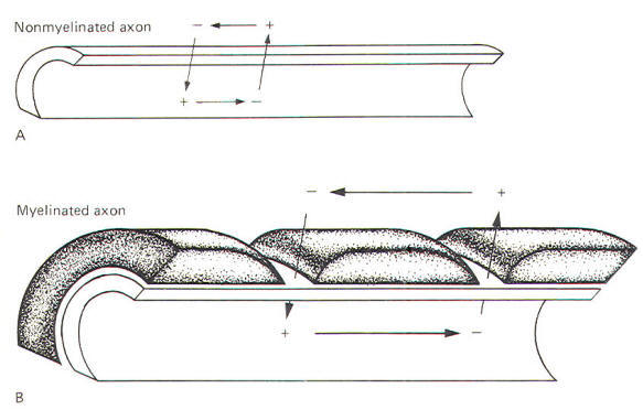
Myelinated neurons propagate action potentials with the same kinds of ion movements as the nonmyelinated neurons just described. The fundamental difference is that the local current flows through the membrane only at the nodes of Ranvier. These nodes are the interruptions in the sheath which surrounds the axons of all myelinated neurons. Current flows through the membrane only at these nodes because they represent areas of relatively low electrical resistance, while the myelinated internodes offer relatively high resistance to current flow. Consequently, when a myelinated neuron is stimulated and an action potential is generated, the local current which flows through the adjacent axoplasm will pass out through the first node rather than through the next adjacent area of membrane. A comparison of the nature of local current flow in myelinated and nonmyelinated axons is illustrated in Fig-14.
In a nonmyelinated neuron the local current must depolarize each adjacent area of membrane - a relatively time-consuming process. Since the impulse proceeds only as rapidly as the spread of the local current, this need to depolarize each adjacent area of membrane imposes necessary restrictions on the conduction velocity. Myelinated neurons, on the other hand, have an advantage which enables them to conduct impulses with a much higher velocity. Since the local current does not need to depolarize each adjacent area of the membrane, impulses travel along the axon at a greatly accelerated velocity. This is called saltatory conduction.
Conduction velocity is roughly proportional to fiber diameter. The greater the diameter of the axon, the greater the conduction velocity. This is true because the larger the diameter, the greater the cross-sectional area of the axoplasm and hence the lower its electrical resistance. Thus a large local current will spread further along the axoplasm before flowing outward through the membrane to complete the circuit. Consequently a greater length of axonal membrane will be depolarized faster, and action potentials will be propagated at a greater velocity. If we think of a length of axon as having a uniform cross-sectional area, the internal axoplasmic resistance to current flow can be calculated using the same assumptions underlying resistance in a length of wire. Ri= ri /π (radius)2 where Ri= axoplasmic resistance per unit length of axon, Ω /cm ri = axoplasmic resistivity, Ω /cm radius = radius of axon, cm
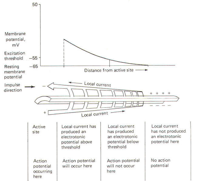
An important point to consider is that one action potential cannot propagate a second without the contribution of the local current. Thus it is clear that the local current plays a crucial role in the impulse conduction process. Current flow in the axon has been likened to current flow in a large undersea cable. Both are composed of a long conducting core (the axoplasm in the neuron) surrounded by an insulator (the neuronal membrane) and immersed in a large-volume conductor (the neuronal extracellular fluid). The axon, however, behaves as a leaky cable in that current not only flows through the axoplasm but leaks out through the membrane as well. Since the same electrical rules apply to current flow in the cable and in the axon, neurophysiologists often speak of the cable properties of the axon. The current which spreads with the impulse is an active current. The local current which we have been discussing is, by contrast, a passive current, and its spread depends only on electrical parameters of the conducting material such as the resistance and capacitance of a unit length of axon. These passive or cable properties of the axon determine the extent and magnitude of the local current. The local current spreads only a very short distance through the axoplasm before flowing out through the membrane, partially depolarizing it, and producing an electrotonic potential (Fig-19). Electrotonic potentials can be observed only when the degree of stimulation is subthreshold because once the excitation threshold is reached the small electrotonic potential is obliterated by the large potential changes associated with the much larger action potential.
The electrotonic potential is the difference between the subthreshold membrane potential at any given time and the resting membrane potential. As action potentials are propagated down the axon, local currents can be visualized as preceding them, depolarizing each newly encountered resting membrane segment and establishing electrotonic potentials which reach threshold and produce additional action potentials (Fig-15).
It is often helpful to picture the membrane and surrounding fluids as an electrical circuit in order to understand the local current flow and the electrotonic potential which it produces. Researchers alike are indebted to the work of Hodgkin for our electrical models of the axon. He pictured the membrane as composed of an infinite number of electrotonic "patches" with each patch composed of a resistance and capacitance in parallel surrounded by intracellular and extracellular fluids, both offering series resistance to the flow of the local current (Fig-16).
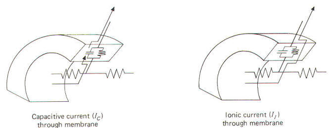
Electrically, the membrane can be thought of as a resistance and capacitance in parallel. The membrane resistance RM represents the difficulty encountered by ions in diffusing through their respective membrane channels, while the membrane capacitance CM represents the charge which exists across the membrane at any time. Now remember that current flow in biological systems consists of moving charges carried by ions. Therefore both capacitive and ionic currents represent the flow of ionic charge. Ionic current II is the charge carried by ions as they flow through their respective ionic channels in the membrane. The difficulty they encounter in passing through these channels from one side of the membrane to the other is represented by the membrane resistance RM . Capacitive current Ic, on the other hand, does not represent the actual flow of ions through the membrane. Its explanation is a little more subtle. If positive ions flow through the axoplasm to the inside of the membrane they will neutralize some of the negative ions already there. This will free some of the positive ions from the immediate membrane exterior to flow away since they are no longer held to the membrane capacitor. Thus positive ions have moved up to and away from the membrane. Thus current has, in effect, traveled outward through the membrane even though no actual ions have crossed from one side to the other. Remember that capacitive current Ic flows only while a capacitor is being charged or discharged. Ionic and capacitive currents are illustrated in Fig-17.
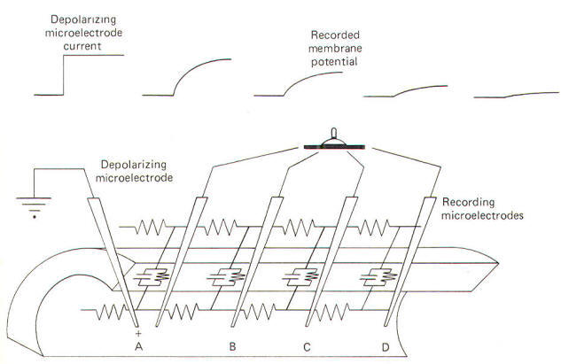
When the local membrane site undergoes an action potential, a local current flows which establishes an electrotonic potential on the next adjacent area of membrane. When this electrotonic potential reaches the excitation threshold, gNa+ will suddenly increase and a second action potential will be generated, obliterating the electrotonic potential and the local current. Unfortunately for experimenters, action potentials propagate so quickly that there is not sufficient time to study the local current itself. However, if the membrane is stimulated to a subthreshold level and held there, the nature and time course of the local current can be studied. A convenient way to do this is to penetrate an axon with a depolarizing microelectrode. In this way a steady but subthreshold level of depolarizing (positive) current can be released internally. By keeping the level of stimulation steady and subthreshold, and by recording the potential changes of the membrane at various distances from the stimulating site, one can examine the magnitude, distance, and time course of the local current spread. Consider the membrane circuit pictured in Fig-18. A depolarizing microelectrode has been placed into the axoplasm at patch A while recording microelectrodes have been inserted at patches B, C, and D. Assume that a steady subthreshold depolarizing current is applied at patch A. A local current will now flow from the less negative region near the tip of the depolarizing microelectrode to the still polarized (more negative) regions of axoplasm at patches B, C, and D before flowing out through the membrane to complete the circuit.
From previous discussions we know that current flow through the membrane is both capacitive and ionic. Both kinds flow in the above circuit. When current is first applied to the axoplasm at patch A, most of it initially goes toward discharging the CM at patch A. Hence Ic flows outward through the membrane at patch A. Initially no II flows outward through patch A because there is no net driving force across the membrane. But as the transmembrane potential is altered from its resting level (RMP) and an electrotonic potential is developed, a net driving force is built up across the membrane. Once the membrane capacitor at patch A has been charged up to the level of the steady depolarizing current at patch A, Ic stops and subsequent current flow outward through the membrane at patch A is purely ionic (II). Not all current from the depolarizing microelectrode becomes outward Ic and II at patch A. Some, progressively less, continues to flow through the internal axoplasmic resistance Ri to first become capacitive and then ionic current through membrane patches B, C, and D. Because voltage drops (decreases) as current flows through increasingly distant lengths of axoplasmic resistance, the membrane capacitors at patches B, C, and D are progressively less completely discharged and exhibit smaller and smaller electrotonic potentials. This is illustrated by the progressively decreased voltage changes recorded by electrodes at patches B, C, and D. Remember that current follows the path of least resistance; therefore, most of the current flows out through the membrane at patch A with progressively less reaching and subsequently traversing more distant points on the membrane. At sufficiently great distances, beyond the reach of the local current, no electrotonic potential is established and the resting membrane potential remains undisturbed.
The electrotonic potential decreases exponentially with distance from the active (stimulated) site according to a value which is known as the length constant λ. λ = [RM/ (Ri + Re)]1/2 where λ = length constant [the distance over which the electrotonic potential decreases to 1/e (37 percent) of its maximum value], cm RM = membrane resistance per unit length of axon, Ω.cm Ri = axoplasmic resistance per unit length of axon, Ω/cm Re = extracellular fluid resistance per unit length of axon, Ω/cm Because of the relatively large volume of the extracellular fluid, its resistance to current flow is very small and can effectively be removed from the above equation, leaving the simple relationship below. λ = ( RM/ Ri)1/2 The length constant is a measure of how far the local current spreads along the axon in front of the action potential. Remember that action potentials give rise to local currents in vivo, while in the experimental situation just described, the depolarizing microelectrode gave rise to the local current. In any case, the longer the length constant the farther the local current will spread through the axon, producing progressively smaller electrotonic potentials before it dies out. Let's now examine those factors which determine the values of RM and Ri since these determine the value of the length constant. If we think of a length of axon as having a uniform cross-sectional area, we can calculate Ri as follows: Ri = ri /π(radius)2 where Ri = axoplasmic resistance per unit length of axon, Ω/cm ri = axoplasmic resistivity, Ω.cm radius = radius of axon, cm The transverse resistance through the membrane for a given length of axon is: RM = rM / 2π(radius) where RM = membrane resistance per unit length of axon, Ω/cm rM = specific membrane resistance, Ω/cm2 Notice that increasing the radius of the axon decreases both the Ri and RM but there is a greater proportional decrease in Ri . Consequently the length constant increases with axon diameter. A long length constant means that larger segments of adjacent membrane will be depolarized faster. Thus as, already pointed out, the larger the axon diameter, the greater the impulse conduction velocity. Most of the aspects of the local current are illustrated in Fig-19.
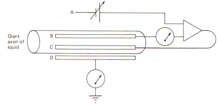
You should be thoroughly familiar now with the relationship between the local current and the action potential. You should also be aware that when the action potential is initiated, several membrane variables change rapidly as a function of time. These are potential, conductance, and current. Now remember that the Ohm's law relationship between them is expressed by: g=I/V where g = conductance, S I = current, A V = potential, V Examination of this relationship shows that g varies as a function of I and V. Hodgkin and Huxley set out to determine the changes in membrane conductance gM during the action potential. Their problem was that both the membrane current lM and the membrane potential VM are also changing constantly during the action potential. Now if one of these variables could be held constant during the action potential (i.e., VM), measurement of lM would enable them to calculate gM at any instant. This is what the voltage clamp technique enabled them to do. A voltage clamp setup is diagrammatically illustrated in Fig-20.
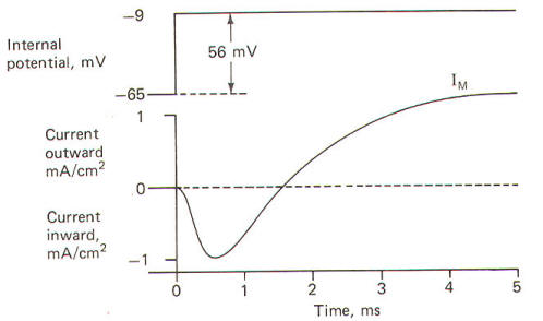
The system operates like this. The experimenter decides on a voltage he would like to produce across the membrane and then sets this "command voltage" on an external voltage source at A (VA). The voltage recording microelectrode at B detects whatever voltage presently exists across the membrane (VB) and sends this signal into the differential amplifier. The signal from the command voltage source is also transferred into the differential amplifier. Now a differential amplifier produces no output if the voltages on its two inputs are equal (VA = VB). But if they are not equal (VA ≠ VB), the amplifier will send whatever current is necessary into the intracellular current-passing electrode at C in order to change the membrane voltage recorded by the recording microelectrode at B until it equals the command voltage. As soon as VA equals VB, the amplifier stops its output. The differential amplifier effectively alters the voltage across the membrane by sending a current through the membrane from the current-passing electrode to the current-recording electrode at D. In the course of crossing a membrane, current discharges the membrane capacitor and hence the membrane voltage. This altered voltage is sent to the differential amplifier for comparison with the command voltage. Consequently the experimenter can "dial" any desired voltage across the membrane, and even more importantly, hold the membrane potential at that level. Now let's examine an experimental situation. Suppose that the RMP of a giant squid axon is -65 mV and the experimenter wishes to "clamp" the voltage at -9 mV. The command voltage is first set at -9 mV. Within microseconds of applying the command voltage, the differential amplifier will pass sufficient current through the membrane to lower the RMP by 56 mV to the set level of -9 mV. Since the membrane potential has now greatly exceeded the excitation threshold, the Na+ channels open, but because of the voltage clamp no actual change in membrane potential is observed. Nevertheless, Na+ ions diffuse inward down their chemical gradient. As they do so, the differential varies its current output proportionally to prevent the Na+ inflow from altering the condition which the amplifier is designed to preserve (VA = VB). Slightly later the K+ channels open and the differential amplifier once again varies its current output proportionally to prevent the K+ outflow from altering the clamped condition (VA = VB). It only takes a few microseconds for the voltage clamp to fix the membrane potential at -9 mV once the command voltage is first applied. Therefore, any subsequent current changes detected by the current-detecting electrode (D) are in response to, and in the opposite direction from, any ionic currents crossing the membrane with Na+ inflow and K+ outflow. The results obtained by Hodgkin and Huxley when they depolarized the membrane of the squid giant axon by 56 mV are pictured in Fig-21. Notice that the membrane current IM is first inward (presumably carried by Na+) and then outward (presumably carried by K+).
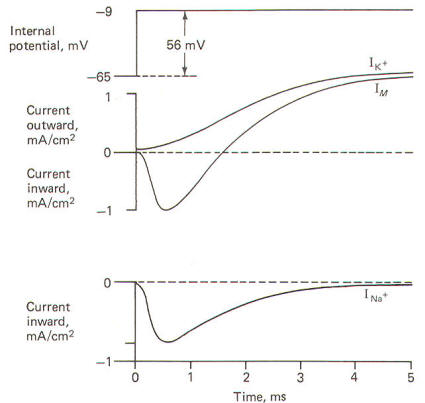
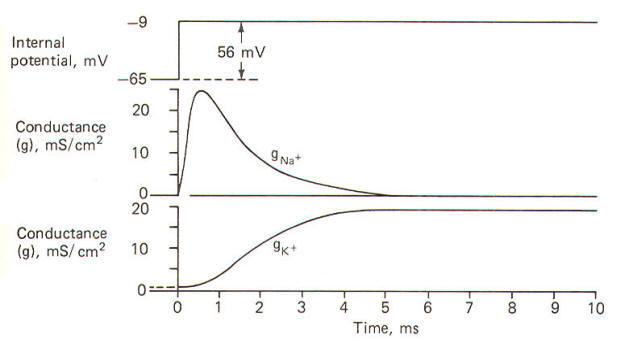
When the squid giant axon is bathed by seawater, a solution similar to its extracellular fluid, and then stimulated to its excitation threshold, the IM is first directed inward and then outward (Fig-22). The contribution of Na+ to the IM could conceivably be eliminated if the extracellular Na+ were reduced to the level of the axoplasm, as this would eliminate the chemical gradient which powers the inflow. Hodgkin and Huxley did this and obtained the results in Fig-22. Notice that following the reduction of the extracellular Na+ to axoplasmic levels, the current flow following stimulation only has an outward component. This current is presumably due almost exclusively to K+ outflow and represents the potassium current IK+. Accordingly, the sodium current INa+ is calculated by subtracting the IK+ from the IM. Presumably IM = IK+ - INa+. Once they had recorded individual ionic currents against a fixed voltage, it was a simple matter using Ohm's law to mathematically calculate individual ionic conductances and then plot them as a function of time. They developed the following equations to do this and then plotted the results in Fig-23.
gion= Iion /(VM - Eion ) gK+ =IK+ /(VM-EK+) gNa+ =INa+/( VM-ENa+) where gion = ionic conduction, µmS/cm2 Iion = ionic current, mA/cm2 VM = membrane potential, mV Eion = ionic equilibrium potential, mV
One action potential propagates a second by means of the local current. The local current depolarizes the adjacent membrane to the excitation threshold at which point rapid but reversible changes occur in gNa+, INa+, and IK+, resulting in the familiar action potential. Fig-24 illustrates the time course of all these events occurring at a single finite location as they were calculated by Hodgkin and Huxley for the data they collected with the voltage clamp experiments.
|
|
|

Copyright [2007] [CNS Clinic-Jordan]. All rights reserved